On Singular Value Decomposition

a small self-note on SVD

Definition

It is way of decomposition any given matrix $ A \in \mathbb{R}^{m \times n} $ into three components which are given as:

\[A = U \Sigma V^T\]

where:

• $ U \in \mathbb{R}^{m \times m} $ is an orthogonal matrix ($U^{T}U = I$)
• $ V \in \mathbb{R}^{n \times n} $ is an orthogonal matrix ($V^{T}V = I$)
• $ \Sigma \in \mathbb{R}^{m \times n} $ is a diagonal matrix with non-negative real numbers (called singular values) on the diagonal

The singular values in $ \Sigma $ are sorted in decreasing order:

\[\sigma_1 \ge \sigma_2 \ge \dots \ge \sigma_r > 0\]

where $ r = \text{rank}(A) $, and the remaining diagonal entries are 0

Remember: Maximum rank of $ A \in \mathbb{R}^{m \times n} $ can be $ \text{min}(m,n)$

\[\underbrace{ \begin{bmatrix} \phantom{0} & \phantom{0} & \phantom{0} & \phantom{0} \\ \phantom{0} & \phantom{0} & \phantom{0} & \phantom{0} \\ \phantom{0} & \phantom{0} & \phantom{0} & \phantom{0} \\ \phantom{0} & \phantom{0} & \phantom{0} & \phantom{0} \\ \phantom{0} & \phantom{0} & \phantom{0} & \phantom{0} \\ \phantom{0} & \phantom{0} & \phantom{0} & \phantom{0} \end{bmatrix} }_{A\ (m \times n)} = \underbrace{ \begin{bmatrix} \phantom{0} & \phantom{0} & \phantom{0} & \phantom{0} \\ \phantom{0} & \phantom{0} & \phantom{0} & \phantom{0} \\ \phantom{0} & \phantom{0} & \phantom{0} & \phantom{0} \\ \phantom{0} & \phantom{0} & \phantom{0} & \phantom{0} \end{bmatrix} }_{U\ (m \times m)} \underbrace{ \begin{bmatrix} \sigma_1 & 0 & 0 \\ 0 & \ddots & 0 \\ 0 & 0 & \sigma_{r} \\ 0 & 0 & 0 \\ 0 & 0 & 0 \end{bmatrix} }_{\Sigma\ (m \times n)} \underbrace{ \begin{bmatrix} \phantom{0} & \phantom{0} \\ \phantom{0} & \phantom{0} \end{bmatrix} }_{V^{T}\ (n \times n)}\]

Geometric Interpretation

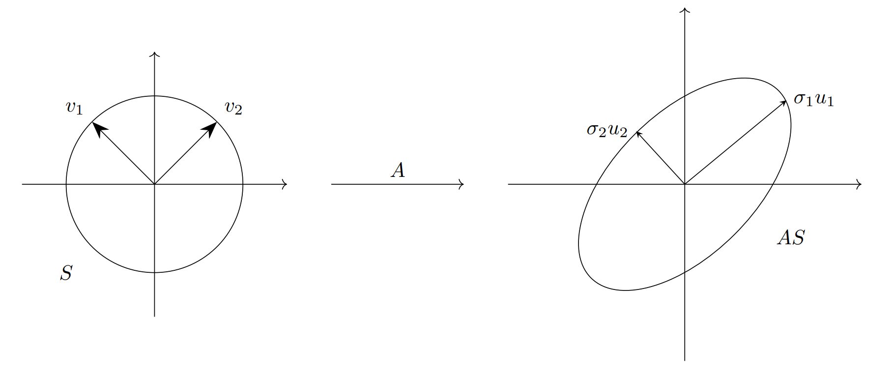
We use the following geometric fact that:

The image of the unit sphere under any $m \times n$ matrix is a hyperellipse.

Let $S$ be the unit sphere in $\mathbb{R}^n$, and take any $A \in \mathbb{R}^{m \times n}$ with $m \geq n$. For simplicity, we take that $A$ has full rank $n$. The image $AS$ is a hyperellipse in $\mathbb{R}^m$. Now, the $n$ singular values of $A$ are the lengths of the $n$ principal semiaxes of $AS$, written $\sigma_1, \sigma_2, \ldots, \sigma_n$. The $n$ ‘left singular’ vectors of $A$ unit vectors ${u_1, u_2, \ldots, u_n}$ are oriented in the directions of the principal semiaxes of $AS$. The $n$ ‘right singular’ vectors of $A$ are the unit vectors ${v_1, v_2, \ldots, v_n} \in S$ so that $Av_j = \sigma_j u_j$. These $v_j$ and $u_j$ are the vectors which are arranged column-wise in the matrices $V$ and $U$.

SVD of a $2 \times 2$ matrix.

Image Compression

One application of Singular Value Decomposition is for image compression. A grayscale image can be represented as a matrix $A \in \mathbb{R}^{m \times n}$, where each element $a_{ij}$ corresponds to the intensity (0–255) of a pixel.

\[A_{m \times n} = U_{m \times m}\, \Sigma_{m \times n}\, V_{n \times n}^{T}\]

Let’s take an example image which has $500$ singular values for its original grayscale form.

Original grayscale image.

Now, we can approximate $A$ by keeping only the top $k$ singular values and their corresponding singular vectors.
This gives a $\text{rank}-k$ approximation:

\[A_k = U_k \Sigma_k V_k^T\]

where:

• $U_k \in \mathbb{R}^{m \times k}$ contains the first $k$ columns of $U$
• $\Sigma_k \in \mathbb{R}^{k \times k}$ contains the top $k$ singular values
• $V_k \in \mathbb{R}^{n \times k}$ contains the first $k$ columns of $V$

The original matrix requires storing $(m \times n)$ values but with the SVD approximation:

If $k \ll \min(m,n):$

Total values stored $= mk + k + nk = k(m + n + 1)$ which is $\ll (m \times n)$

For much smaller value of $k$ (in comparison to the original number of singular values which is $500$ in this case), much of the features of the original image are preserved.

Reconstructed images.

Here, $\text{RE}$ stands for Reconstruction Error which is found by taking the Mean Squared Error between the original and the reconstructed image.